
Why do certain channels on a mixing console featuring transient signals (like drums) run hotter than other channels (e.g., strings) even though they all sound equally loud? Let us look at duty cycles.
In Part 1 of this article‑series we looked at the defention of crest factor and how to calculate it. In Part 2 we studied the effect of filtering on crest factor. And in this article — Part 3 — we will look at duty cycles.
A duty cycle is the fraction of a period during which a signal is active. Where one period is the time it takes for a signal to complete an on‑and‑off cycle.
Duty cycle is commonly expressed as a unitless percentage or a ratio. As a formula, a duty cycle (%) may be expressed as shown in Equation 1:
\begin{equation}D=\frac{t_{on}}{\left ( t_{on}+t_{off} \right )}\times100\%\end{equation}
Where \(t_{on}\) is the duration during which the signal is switched on, whereas \(t_{off}\) is the duration during which the signal is switched off. 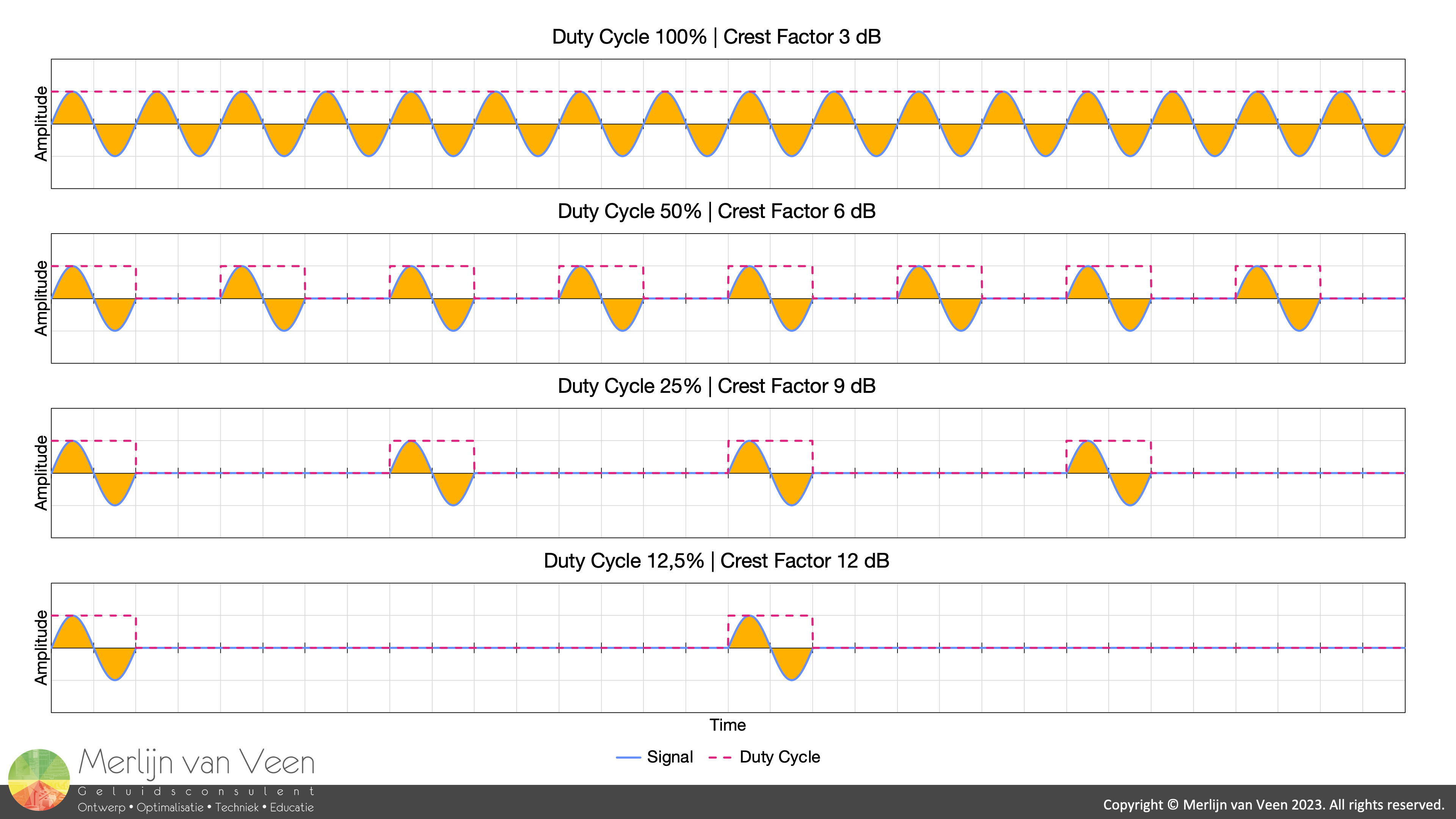 Figure 1Figure 1 shows four scenarios for a sine wave where the duty cycle is reduced from 100% to 12,5%.
Since an RMS‑level's corresponding signal power is proportional to the area underneath the waveform (shaded in orange color). Each time the duty cycle is halved, area is halved as well, i.e., signal power is halved, and the RMS‑level drops by 3 dB.
Notice in Figure 1 that peak levels remain identical regardless of duty cycle. As a result, for each halving of the duty cycle, the base‑signal's crest factor (3 dB for a sine wave) is increased by 3 dB.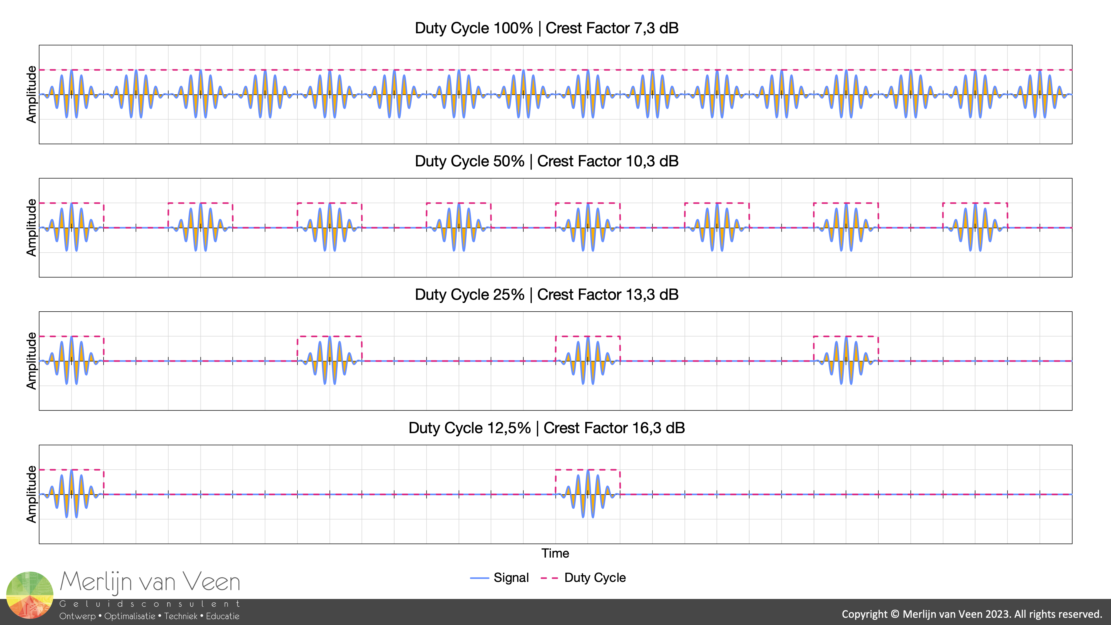 Figure 2This is also true for the — gated — sine wave (aka tone burst) in Figure 2. Except that the crest factor for a gated sine wave (also when played end‑to‑end) is no longer 3 dB to begin with, but 7,3 dB.
Regardless, each time duty cycle is halved, crest factor rises by 3 dB as well. Which also goes for noise signals.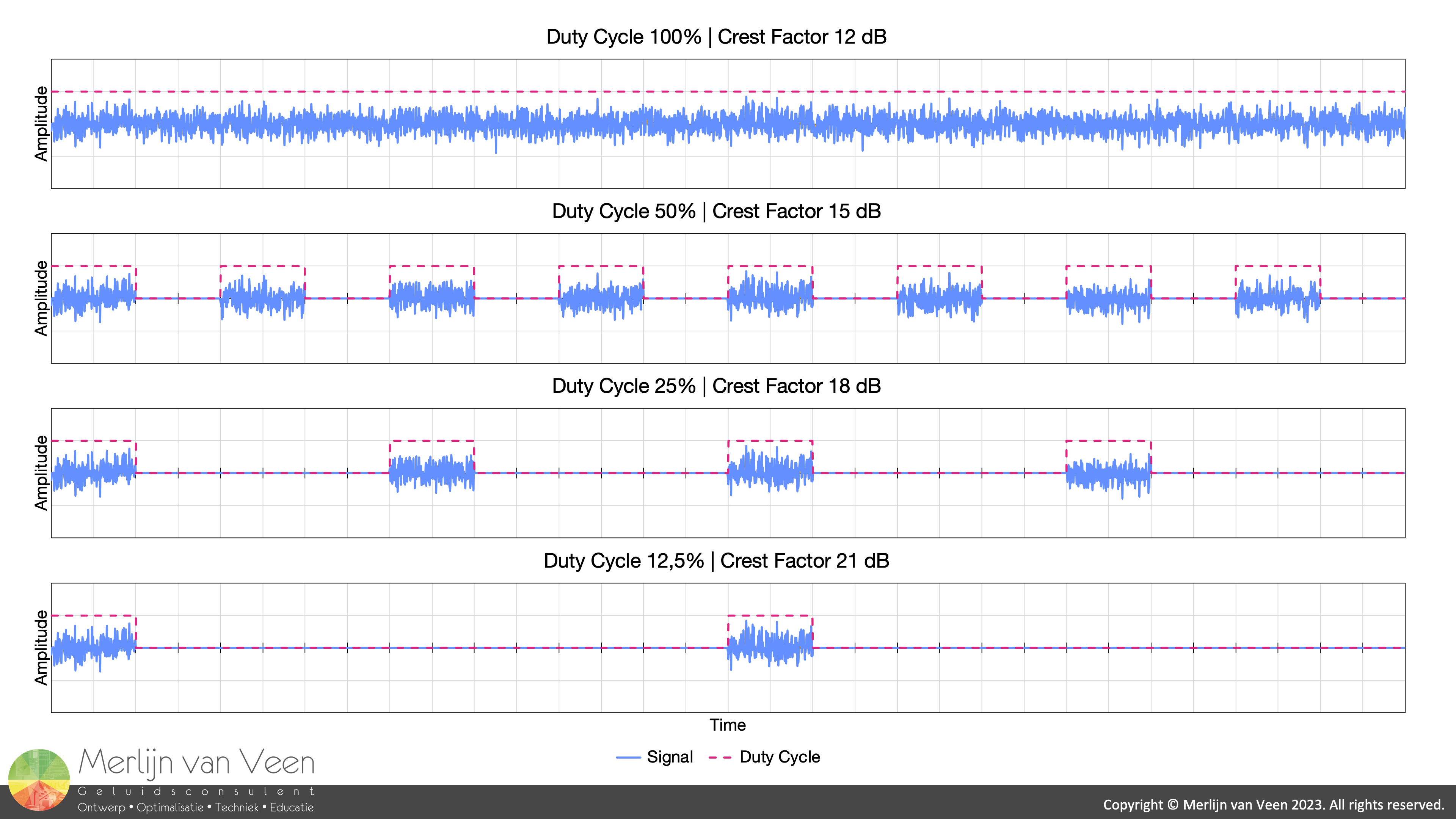 Figure 3Figure 3 shows noise as the base‑signal whose inherent crest factor is 12 dB.
Notice once more that, crest factor rises by 3 dB every time the duty cycle is halved.
These three examples show that every time a signal becomes sparser, with increasing downtime between consecutive events, crest factor rises.
Hence the metaphor: "Crest Factor is the difference between how hard one hits a drum and how often one hits the drum". Where "hard" (read: intensity) determines the peak level and "often", i.e., the number of hits per time‑interval, determines the average level.
RMS‑Normalized results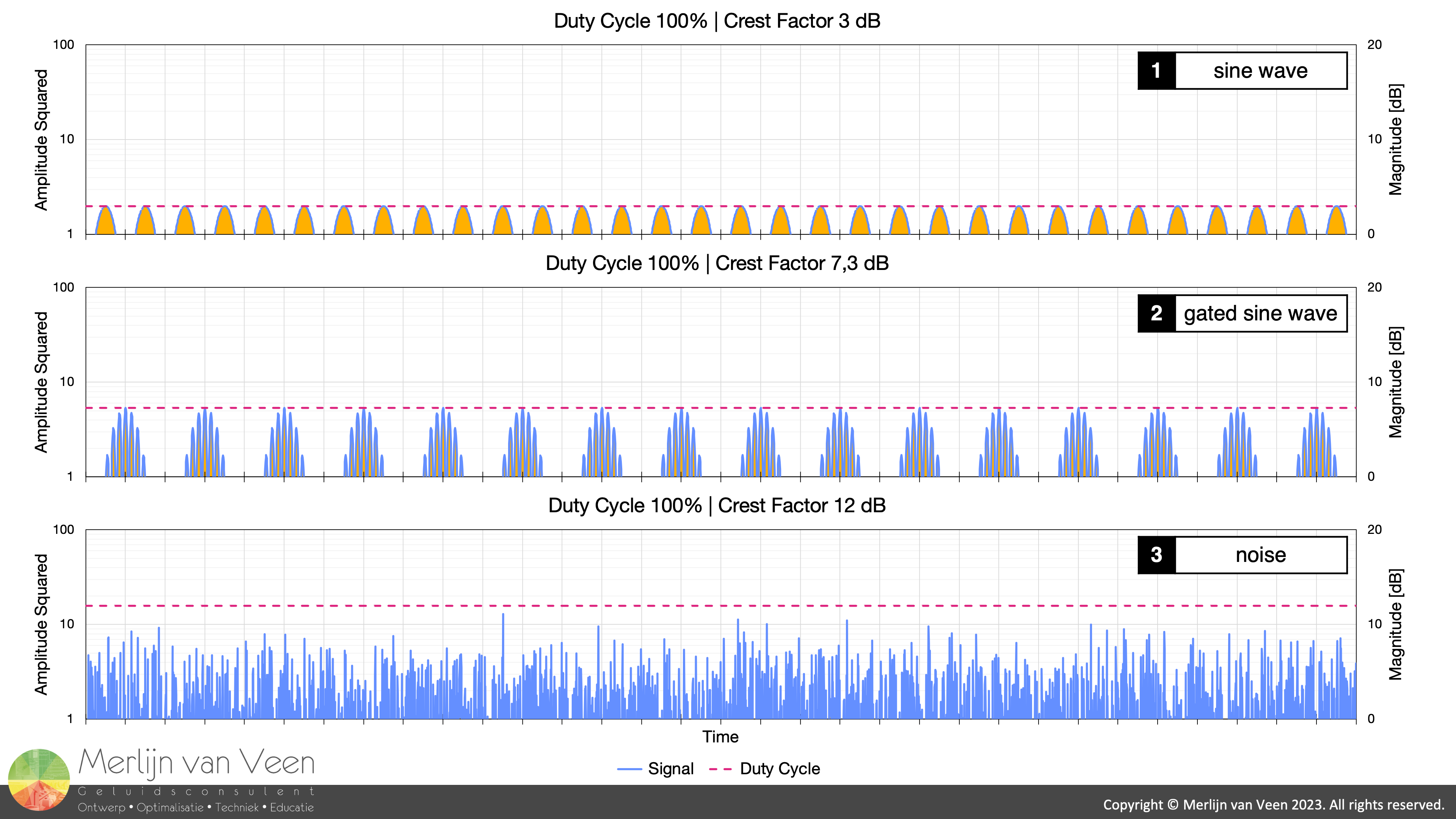 Figure 4
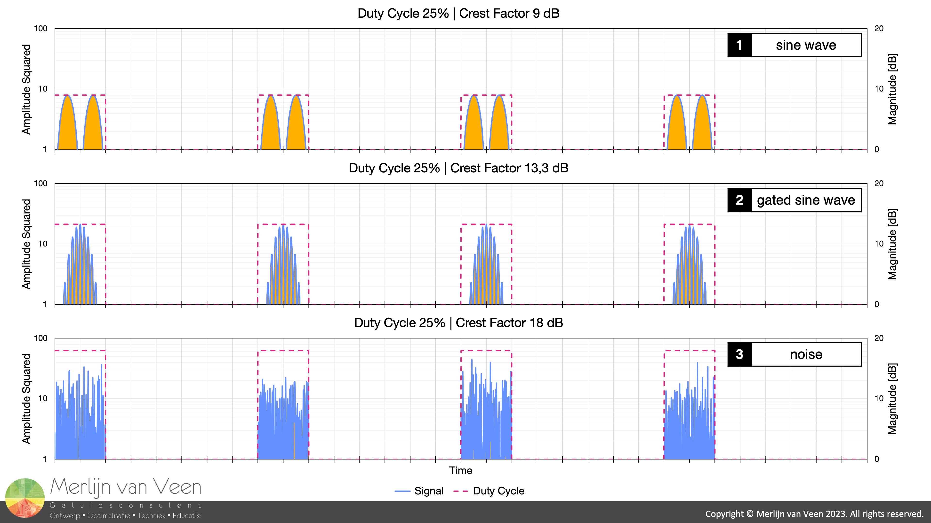 Figure 5So far, we have been looking only at peak‑normalized results. However, the perception of loudness is closely related to RMS levels as opposed to peak levels. As such, Figures 4 and 5 show RMS‑normalized results for two duty cycles and all three signals.
Unsurprisingly, Figure 4 shows that all three signals, at some arbitrary albeit identical nominal level, with 100% duty cycle, require different amounts of — peak room — to pass through the signal chain. This is exacerbated by decreasing the duty cycle.
Figure 5 shows the same three signals with a 25% duty cycle.
Notice that the noise signal in Figure 5.3 requires — 15 dB more — peak room, at the same nominal level, than the continuous sine wave in Figure 4.1.
Which sheds some light on why some signals run hotter on a mixing console than others, even though they sound equally loud.
Caution with geusstimating peak levels
None of this comes easy (at least not to the author) and caution is required when — calculating (rather than measuring) — peak levels from RMS levels. Whether they be time‑weighted (fast or slow) or time‑averaged (Leq) sound levels.
The author is aware of two common instances where false assumptions are known to be made.
Case #1
AudioXpress magazine featured an article in 2021 on the ANSI/CTA‑2010 Standard (based on work done by Don Keele). An interesting standard that uses tone bursts for rating subwoofer‑output while considering auditory masking of harmonic distortion.
The article's author made the honest mistake of simply assuming peak levels to live 3 dB higher than measured RMS levels. Since the test involves sine waves albeit gated.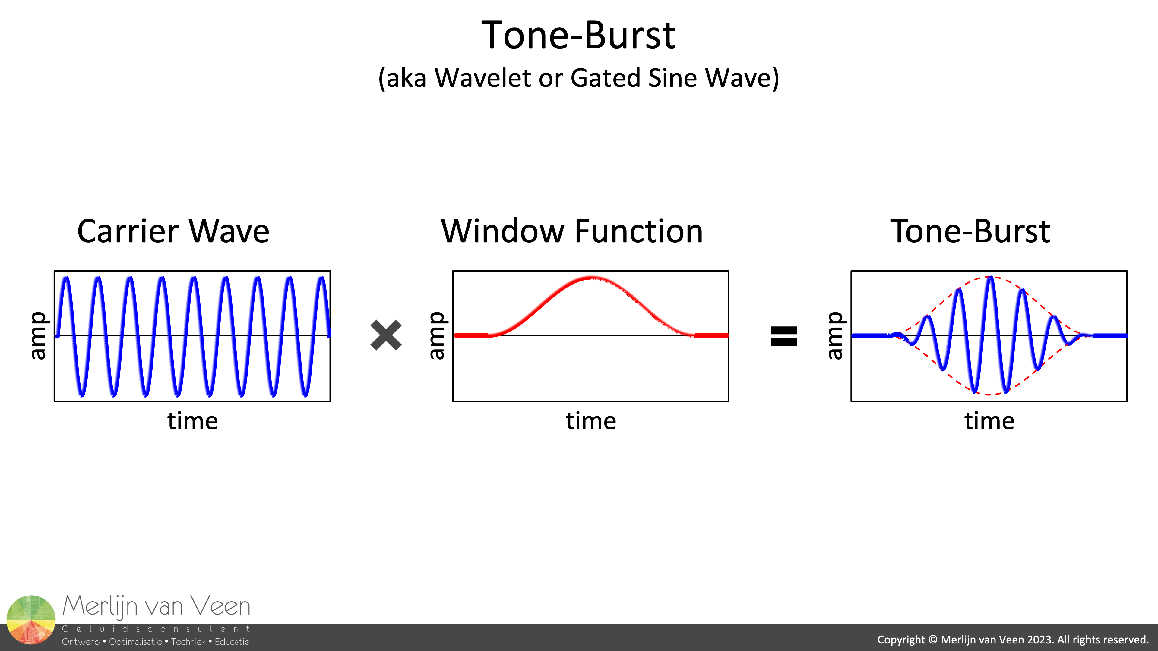 Figure 6Figure 6 shows a tone burst where, by applying an amplitude envelope to a carrier wave, the latter stops being a pure tone and is turned into a band‑limited group of frequencies.
The ANSI/CTA‑2010 Standard uses a 6,5‑cycle‑long carrier wave with a Hann window applied to it.
The resulting waveform can be mathematically described using the piecewise function shown in Equation 2:
\begin{equation}f(t)=\begin{cases}
\color{Red} {\frac{\left \{ 1-cos\left [ \frac{\left (2\pi f_{0}t \right )}{6{,}5} \right ] \right \}}{2}} \color{Blue} {sin\left ( 2\pi f_{0}t \right )} & \text{, for } 0\leqslant t\leqslant \frac{6{,}5}{f_{0}} \\
0 & \text{, elsewhere}
\end{cases}\end{equation}
Where the blue part is the carrier wave and the red part is the Hann amplitude envelope.
The exact RMS level of a sine wave — with an amplitude of one — can be derived using Equation 3:
\begin{equation}\sqrt{\frac{\int_{0}^{2\pi}\left[ \color{blue}{sin(x)} \right ]^2dx}{2\pi}}=\frac{1}{\sqrt{2}}\approx 0{,}707\; \Rightarrow \; -3\, dB\end{equation}
Which (unsurprisingly) turns out to be 3 dB less than its peak level.
Whereas the exact RMS level of a Hann function — with an amplitude of one — can be derived using Equation 4:
\begin{equation}\sqrt{\frac{\int_{0}^{2\pi}\left \{ \color{Red} {\frac{\left [ 1-cos(x) \right ]}{2}} \right \}^2dx}{2\pi}}=\frac{\sqrt{\frac{3}{2}}}{2}\approx 0{,}612\; \Rightarrow \; -4{,}27\, dB\end{equation}
Where the RMS level is 4,27 dB less than its peak level.
The RMS level of a single tone burst — with an amplitude of one — simply equals the product of both the RMS levels of the carrier wave and the amplitude envelope, as shown in Equation 5:
\begin{equation}\color{blue} {\frac{1}{\sqrt{2}}} \times \color{red} {\frac{\sqrt{\frac{3}{2}}}{2}} =\frac{\sqrt{3}}{4}\approx 0{,}433\; \Rightarrow \; -7{,}27\, dB\end{equation}
Where the RMS level is 7,27 dB less than its peak level as opposed to 3 dB, as suggested by the sine wave while ignoring the amplitude envelope!
Notice in Figure 2, this is also true for a series of tone bursts played end‑to‑end (without duty cycle).
Case #2
In Part 2 of the Crest Factor article‑series, it is shown that for "complex" signals — that consist of two or more sinusoidal components — e.g., a square wave or noise, crest factor changes by filtering.
Up until standard AES2‒2012, oftentimes (for pragmatic reasons) soft‑clipped pink noise with a — crest factor of 6 dB (as opposed to 12 dB) — would be used for rating loudspeaker sound levels. Where peak levels were simply — assumed — to be 6 dB higher than the measured average sound levels.
However, once such a low‑crest‑factor signal is passed through a loudspeaker system — which invariably acts like a filter — it becomes unorganized, and its crest factor tends to 12 dB again. In most cases, the peak levels gain market share, as opposed to the RMS level loosing market share, where the latter remains virtually constant. Resulting in many under‑estimated peak levels.
Adding insult to injury
In both cases, the false assumptions are prone to even larger errors once one starts to play back the tones or noises in bursts (as opposed to continuously) whereby invoking a duty cycle. Now the number of repetitions per time‑interval, and the subsequent downtime between consecutive bursts, will affect the measured RMS level. Where any and all assumptions about peak levels should be made with great caution.
In stead, it is much better to simply measure peak sound levels (as opposed to guesstimating) using a sound level meter with a "hold" function that records the highest instantaneous peak sound level while the measurement was running.