
In part 2 of this article series, we will explore how filters — that invariably change level or phase as a function of frequency — can affect crest factor. Towards the end, you can download a MS Excel Workbook for free that contains all relevant calculations and graphics used in this article.
During part 1 we saw that crest factor is a waveform's peak‑to‑average ratio where average stands for the quadratic mean, better know as Root Mean Square or RMS.
Easy Start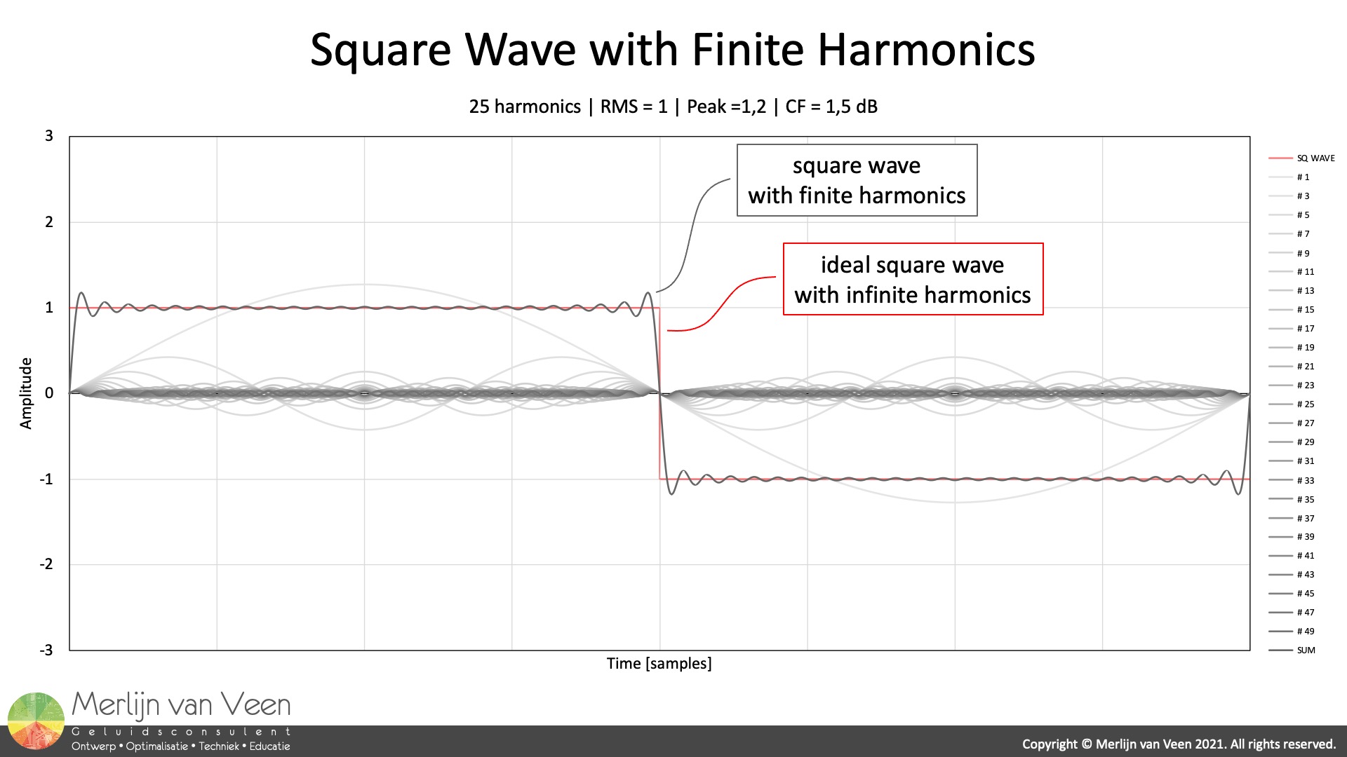 Figure 1To appreciate how filters can affect crest factor, we should take advantage of a familiar starting point: the square wave (Figure 1) with its —well known — crest factor of one.
The square wave will serve as case study for explaining the abstraction. That being said, towards the end I will leave you with enough breadcrumbs to increase your understanding.
An ideal square wave can be represented as an infinite sum of sine wave components.
\begin{equation}x(t)=\frac{4}{\pi }\left [ sin(\omega t)+\frac{1}{3}sin(3\omega t)+\frac{1}{5}sin(5\omega t)+\cdots \right ],\; \; \; \; where\; \omega=2\pi f \end{equation}
Equation 1 shows the recipe for constructing an ideal square wave with an RMS value of one that consists solely of odd‑integer harmonic frequency components.
Gibbs Phenomenon
However, when this infinite harmonic series is truncated, i.e., a finite number of harmonics rather than an infinite amount, which happens in loudspeakers that invariably exhibit low‑pass behavior near the upper limit of human hearing as well as in the digital domain due to the anti‑aliasing (low‑pass) filter, the square wave will exhibit overshoot at the jump discontinuities (Figure 1) known as the Gibbs phenomenon.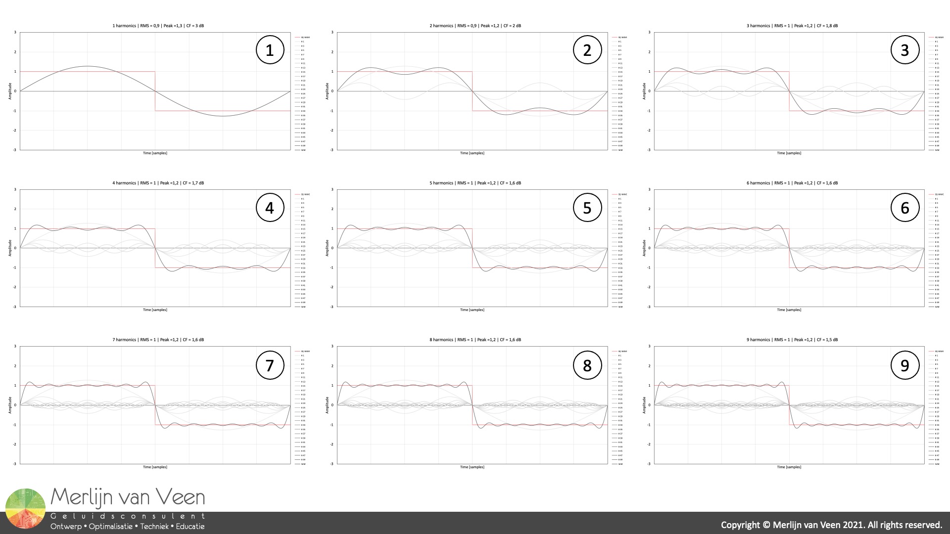 Figure 2Notice in Figure 2 that a square wave approximation improves with each harmonic added.
For the calculation examples in this article, the number of harmonics (including the first harmonic or fundamental frequency) is limited to a maximum of 25. Despite this constraint, the RMS value is indeed one; however, due to the Gibbs phenomenon, the peak value is 1,2 (Figure 1) rather than the expected value of one for ideal square waves whose RMS level is one as well.
Consequently, the crest factor for this square wave approximation is not one (on a linear scale) or zero dB (on a logarithmic scale) as is expected of ideal square waves. Nevertheless, if the number of harmonics were to be increased, the Gibbs phenomenon would be minimized and the crest factor is expected to converge towards one or zero dB.
It is all about the Phase
The textbook version of the genuine square wave occurs if and only if each individual sinusoidal component, i.e., harmonic (including the fundamental frequency), has an initial condition of zero‑degrees phase offset. Which raises the question: "What if the harmonics are phase‑offset?" Figure 3Figure 3 shows six instances where the very same sinusoidal components — without changing their amplitudes — have their phases randomized so that they sum to a certain peak value.
What is remarkable is that, in each instance the individual sinusoidal components — despite their randomized phases — sum to the same RMS value albeit with different peak values, i.e., crest factors. Notice that the crest factor starts out with a value of 3 dB and rises all the way to 8 dB.
So far, the most important takeaway is this: All other things being equal, scrambling a square wave's harmonics makes its crest factor rise without exception!
Let us see this in action by filtering an actual square wave.
⚠ CAUTION: LOUD VIDEO FOLLOWING NEXT ⚠
The first example in the video above demonstrates a square wave whose sinusoidal components' phases are rearranged by means of an all‑pass filter which allows "all frequencies to pass", i.e., no attenuation of the harmonics, while introducing — loosely defined — frequency dependent delay, i.e., the harmonics are phase‑offset.
Please pay attention to the following:
- In the time domain (oscilloscope and VU meters):
- The waveform shape changes dramatically
- The waveform's crest (peak) changes dramatically
- The peak level changes accordingly
- Nevertheless, the RMS level remains constant
- In the frequency domain (spectrum analyzer):
- The line spectrum remains identical (between adjustments)
- Sound quality
- No audible changes
The second example in the video demonstrates the effect of a high‑pass filter with a corner frequency of 32 Hz — well below the square wave's fundamental frequency of 187,5 Hz — so that it does not attenuate the harmonics. Regardless — apart from FIR filters — the filter's associated phase shift inevitably rearranges the sinusoidal components' phases and the waveforms's crest (peak) and therefore crest factor rises once more.
DISCLAIMER: Observations like these (but not limited to) lead people to believe that humans are phase deaf; however, the author would like to remind the readership that these specific examples consider — steady‑state signals — whereas for transient/percussive signals phase shift audibility is a different story altogether as you can tell from the next video.
Without digressing too much, each of the three signals in this video consists of the same sinusoidal components — with the same amplitudes — whose phases have been arranged differently. Notice that, unlike for the steady‑state square wave in the previous video, there is an audible difference.
Regardless, the important takeaway is this: All loudspeakers — without exotic processing — invariably act as high‑pass filters (complete with phase shift) which affect square wave reproduction; moreover, low‑pass filter behavior, near the upper limit of human hearing, makes matters even worse.
CAUTION: Should you decide to put this to the test with real loudspeakers, please exercise caution. Square waves at high levels may harm the loudspeaker.
Parseval's Theorem
The behavior observed in the first video is explained more rigorously by Parseval's Theorem which for our application — loosely defined — states: The area underneath a given signal's Power Spectral Density (PSD) in the frequency domain, colloquially referred to as line spectrum, equals the mean area underneath that signal's squared waveform in the time domain.
In the video, the line spectrum — despite rearranging the square wave's sinusoidal components' phases — remained identical (between adjustments) because the component's amplitudes were deliberately left alone. Consequently, the area underneath the line spectrum remained the same as well. When the area underneath the line spectrum is the same, then so is the mean area underneath its squared waveform and since the RMS value is proportional to the latter (Part 1) it remains the same as well even though the peak value and therefore the crest factor did not.
In other words, there are infinite many ways to generate a square wave's frequency spectrum with an atypical crest factor by rearranging the sinusoidal components' phases; however, there is only one way, i.e., no phase‑offset harmonics, to do so with a crest factor of one or zero dB.
Delicate Matters
By now, you can hopefully appreciate that there's is something very delicate about how a given signal's sinusoidal components are organized.
When you randomize the sample order of pink noise it becomes white noise as demonstrated in my article "A Noisy Story".
When you high‑pass low crest factor signals (6 dB or less) such as noise — or music — the crest factor rises significantly as demonstrated in my article "Don't Judge a Booklet by its Cover". The latter happens invariably since every loudspeaker — without exotic processing — acts as a high‑pass filter.
In general, low crest factor signals are more prone to filter‑related crest factor changes, whereas high crest factor signals tend to be more immune.
Free MS Excel Workbook
You can freely download a copy of the MS Excel Workbook used to create Figures 1 through 3 using the link shown below. In the workbook's spreadsheets you can see all calculations in action, change the number of harmonics and randomize the sinusoidal components' phases to attain a particular crest factor.