Crest factor is an important metric associated with phenomena such as (but not limited to) headroom, distortion, instantaneous power consumption, and loudspeaker driver excursion.
In part 1 of this 4‑episode series on crest factor, we will begin by defining crest factor first. Towards the end, you can download a MS Excel Workbook for free that contains all relevant calculations and graphics used in this article.
Subsequent episodes will cover crest factor and filters, crest factor and power consumption, and crest factor in the air: measuring sound levels.
Crest factor is a parameter of a waveform, such as alternating current or sound, showing the ratio of peak values to the effective value.
- Wikipedia -
Colloquially, it is also known as the peak‑to‑average ratio that tells us how far the waveform peaks stray from its average value.
\begin{equation}crest\; factor \propto \frac{peak}{average}\end{equation}
To determine the crest factor, the challenge becomes to first figure out the waveform's "average" which — for our application — we will attempt in two ways.
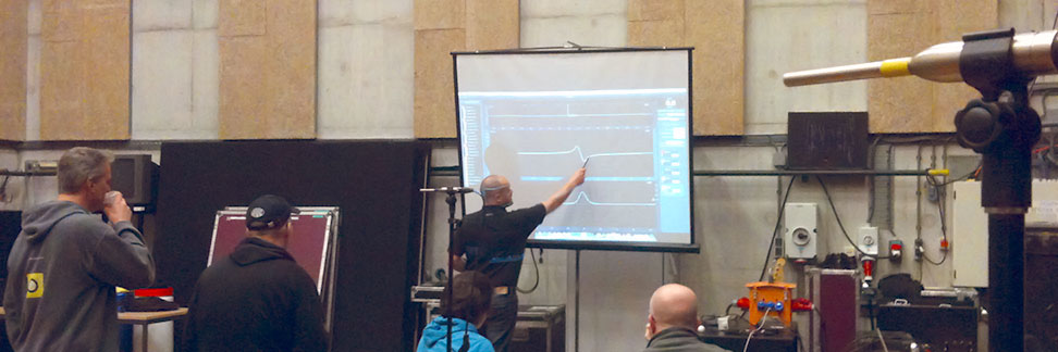
Method #1: Arithmetic Mean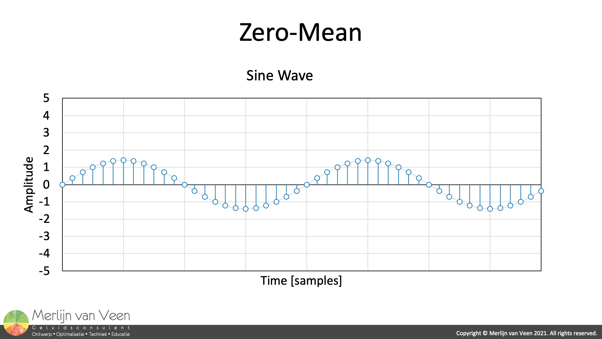 Figure 1For — alternating signals without a DC offset — the arithmetic average is typically zero.
For example, notice for the sine wave in figure 1 that, for each positive value there is an — equally large but opposite value — that nullifies it, hence zero‑mean.
⚠ JOKE FOLLOWING NEXT - DO NOT TRY THIS ⚠
And yet, intuitively we all know that, when we wet our fingers and stick them in the nearest electrical outlet which supplies sinusoidal AC as well, we will not sense zero volts on average.
⚠ END OF JOKE ⚠
Suffices to say, things do not add up or do they? Regardless, we cannot use a value of zero as average for the denominator in Equation 1, because bad things happen when you divide by zero, i.e., a workaround is needed.
However, before we can look at the second averaging method, we have to make a minor detour first.
Root‑Power Quantity or Power Quantity
Our success depends on the measurement unit used for a particular waveform. For our application, the measurement unit is typically associated with pressure or voltage. However, in order for us to move forward, we need "power quantities" rather than "root‑power quantities", formerly known as "field quantities".
A root‑power quantity is a quantity such as voltage, current, or sound pressure,
the square of which, in linear systems, is proportional to power.
The term root‑power quantity refers to the square root
that relates these quantities to power.
The term was introduced in ISO 80000‑1 § Annex C;
it replaces and deprecates the term field quantity.
- Wikipedia -
 Figure 2For sake of simplicity, we will remain in the electrical domain where according to "Joule's law" (Figure 2)
\begin{equation}P = I^2 \times R\end{equation}
power is proportional to current squared, and when we substitute "Ohm's law"
\begin{equation}I= \frac {E}{R}\end{equation}
where current is proportional to voltage, into Joule's law, we get
\begin{equation}P = \frac {E^2}{R}\end{equation}
where power is proportional to voltage squared. Notice that, in either case, i.e., current or voltage, power is proportional to squared values. A proportionality that is harnessed in the second averaging method.
Method #2: Quadratic Mean
Unlike the arithmetic mean, the quadratic mean, colloquially referred to as — Root Mean Square or RMS — will not leave us hanging with an average value of zero.
For alternating electric current, RMS is equal to the value of the constant direct current that would produce the same power dissipation in a resistive load.
- Wikipedia -
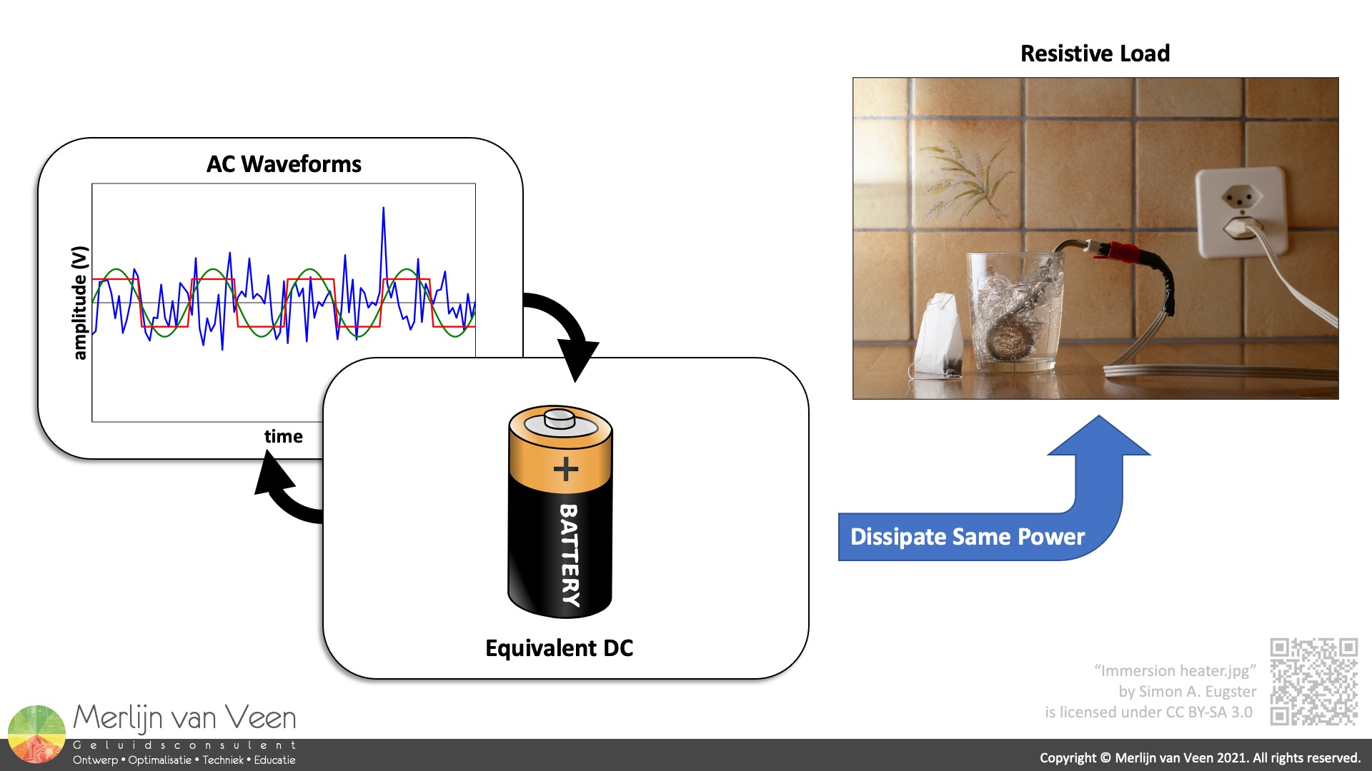 Figure 3In the electrical domain, the outcome can be thought of as the answer to the question (Figure 3): "What voltage rating should a DC source, such as a battery, have to dissipate the same power in a purely resistive load?". This DC‑equivalent value is also known as the "effective" value.
\begin{equation}f_{RMS}=\sqrt{\frac{{\color{Red}{\int_{T_1}^{T_2}\left [ f(t) \right ]^2dt}}}{T_2-T_1}}\end{equation}
For continuous signals, RMS is calculated using Equation 5 which admittedly looks intimidating. However, the sole reason I am showing this equation, is to call attention to the integral in the numerator — where \(f(t)\) represents an arbitrary waveform as a function of time whose values are squared — informing us this will be an exercise in areas underneath squared curves.
\begin{equation}x_{RMS}=\sqrt{\frac{\left ( x_1^2+x_2^2+\cdots +x_n^2 \right )}{n}}\end{equation}
Fortunately, for discrete signals, the math is significantly less intimidating and effectively translates into a 3‑step recipe (Equation 6):
- Square each sample value
Purpose: map the root‑power quantity to a power quantity. - Calculate the Mean
Purpose: calculate the average power‑proportionate value. - Find the square Root
Purpose: map the power quantity back to the initial root‑power quantity.
 Figure 4Figure 4 shows the recipe applied to three different waveforms of the same length (48 samples) — whose arithmetic mean is zero — and have another thing in common; they all have the same RMS value, i.e., the same mean area under their squared curves for the duration of the signals.
Since the squaring operation in Step 1 maps a root‑power quantity to a power quantity where power [J/s] × time [s] = energy [J], the same mean area under the curve (remember the integral from Equation 5) implies same mean energy.
Crest Factor Continued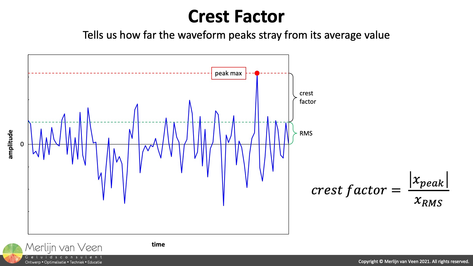 Figure 5Now that we have seen the method for determining an average for alternating signals we can finally calculate the crest factor.
\begin{equation}crest\; factor=\frac{\left | x_{peak} \right |}{x_{RMS}}\end{equation}
Where \(x_{peak}\) is the largest absolute (sign insensitive) value for the duration of the signal (Figure 5).
Going back to Figure 4, you can tell that the crest factor for a sine wave is √2 (roughly 1,41) whereas for the square wave it is one, i.e., no peaks at all. The crest factors for conventional zero‑mean waves such as sine, square, triangle, and sawtooth waves are all constant — albeit different — and well known.
Whereas, colors of noise such as white, pink, and red (or brown) typically have crest factors of about four. In a later episode we will discover there are exceptions.
And while all the signals in Figure 4 have have been calibrated such that they have the same RMS value, their peak values differ by as much as a factor of four. Therefore, the higher the crest factor, the further signal peaks stray from the RMS value.
Bilingual
When it comes to crest factor, audio professionals are expected to be bilingual, i.e., tell the difference between crest factor expressed on a linear or logarithmic scale.
The previous equation provides the linear answer which can easily be converted to dB (logarithmic) by applying the "\(20\times log_{10}\)" rule for root‑power quantities
\begin{equation}20\times log_{10}\left ( \frac{\left | x_{peak} \right |}{x_{RMS}} \right )\end{equation}
whereas the "\(10\times log_{10}\)" rule is exclusive to power quantities. Equation 8 provides the logarithmic answer in dB and yields the following results for the signals in Figure 4.
| Crest Factor (lin) | Crest Factor (log) | |
| Square Wave | 1 | 0 dB |
| Sine Wave | 1,41 | 3 dB |
| Noise | 4 | 12 dB |
RMS and Loudness
RMS is an important metric closely related to loudness. Whether it is time‑weighted or time‑averaged sound levels as defined in the sound level meter standard IEC 61672‑1, or Loudness units such as LKFS (ITU-R BS.1770) or LUFS (EBU R 128), all calculations are based on RMS.
Free MS Excel Workbook
You can freely download a copy of the MS Excel Workbook used to create Figure 4 using the link shown below. In the workbook's spreadsheets you can see all calculations in action, change the amplitude and time period for the sine and square waves, and change the RMS value and crest factor for the noise signal.