 Time and again, I keep reading on the internet that cardioid gradient arrays (also known as CSA), lack impact and suffer from time smearing. I can’t help but feel that this prejudice is unwarranted.
In this article, I will elaborate once more on why this notion might be unjustified.
Gradient arrays go back to at least 1972 when Harry Olson published his paper on the topic at the 43rd AES Convention in New York City. It’s mature theory which unfortunately is still poorly understood.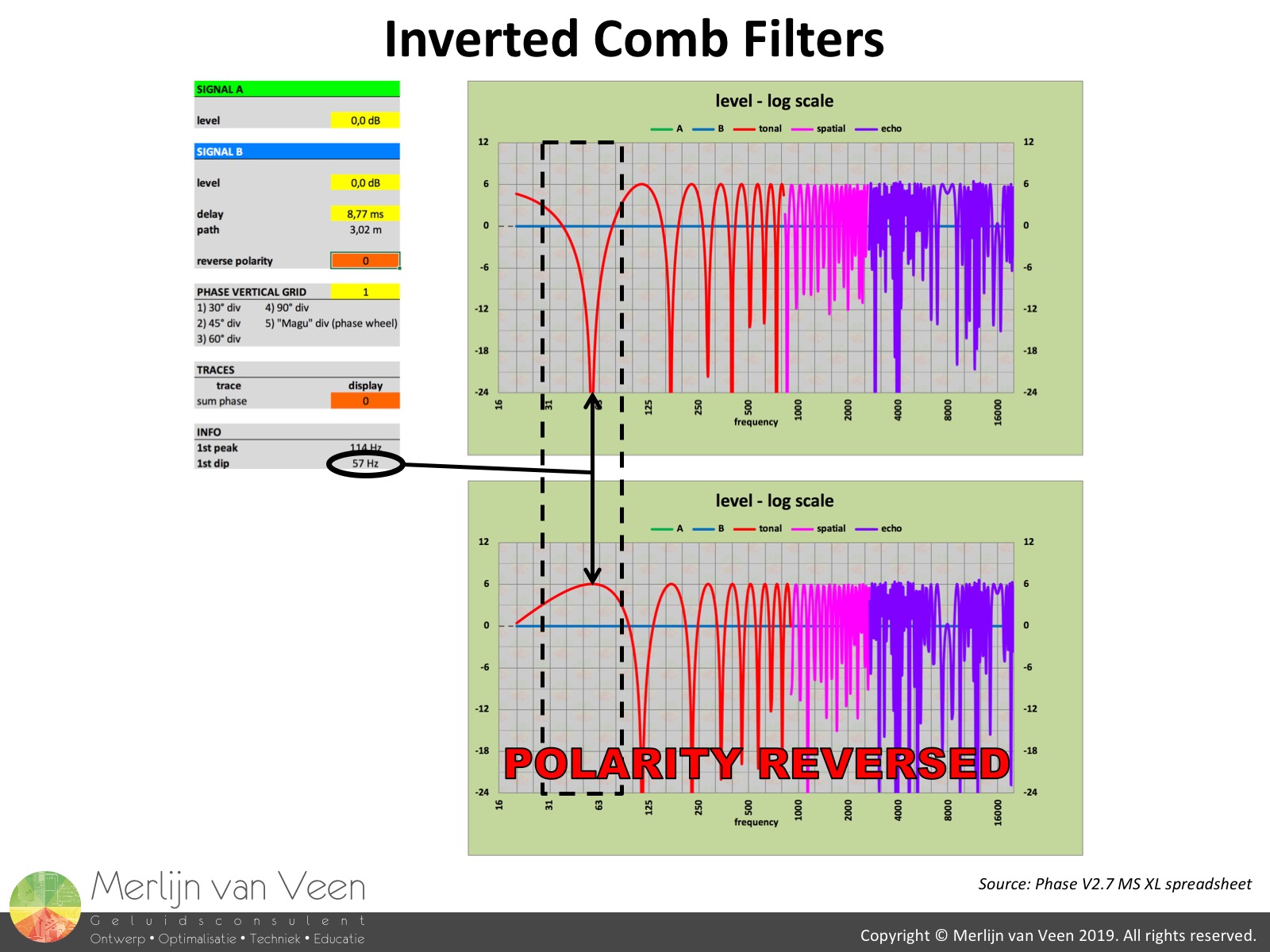 figure 1
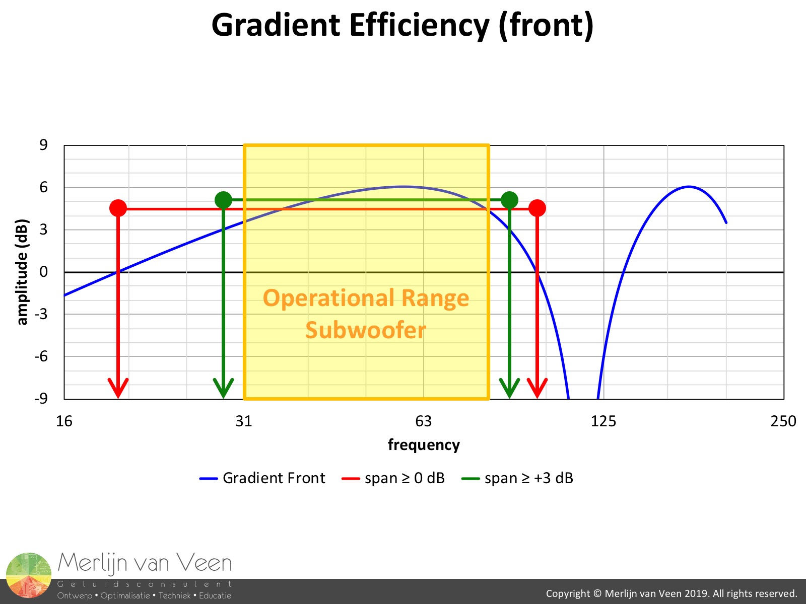 figure 2
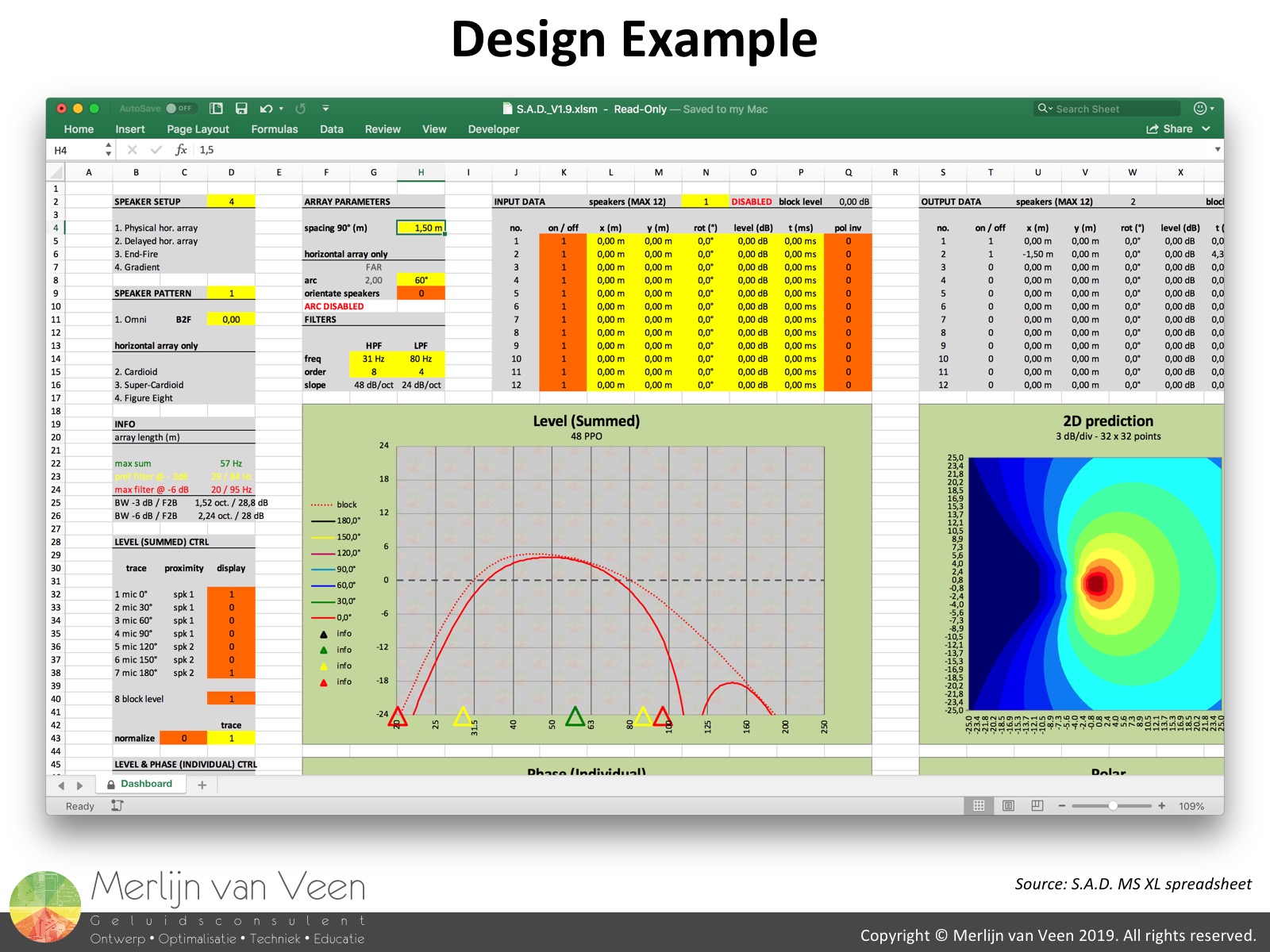 figure 3
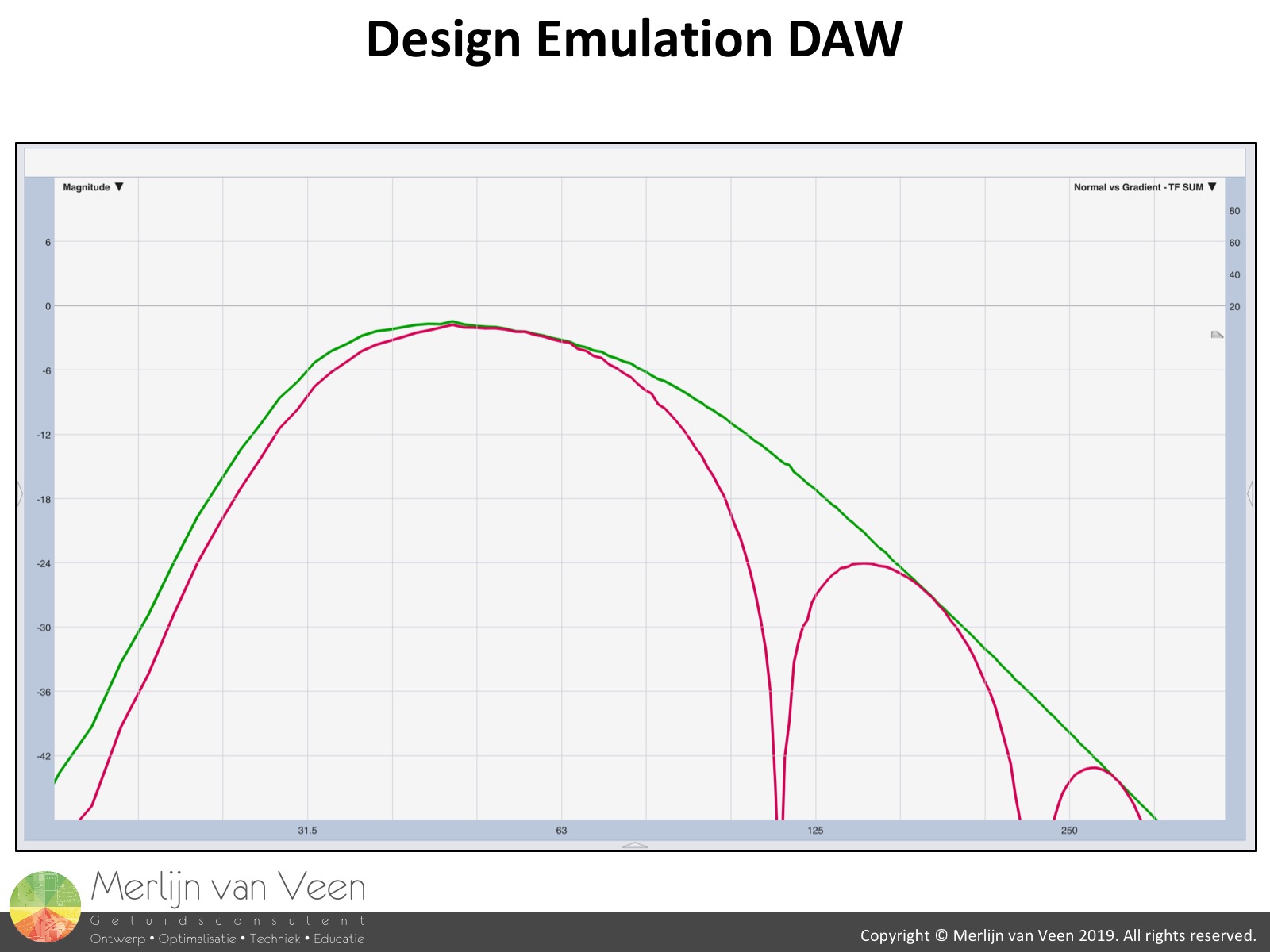 figure 4
 figure 5
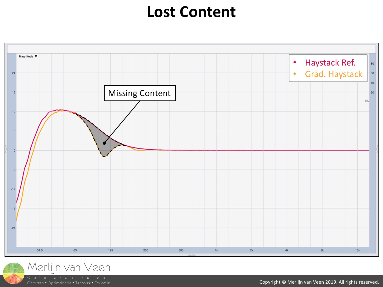 figure 6The principle exploits a comb filter’s first “tooth” or cancel and turns it into a peak with help of a polarity reversal (figure 1). In practice, that peak acts as a band-pass filter with a clearly defined usable bandwidth.
Contrary to end-fire which is easier and more forgiving, the rules of engagement for gradient arrays are much more stringent. But, as long as you respect those rules, you should be fine.
So, in the interest of the SPL-Preservation-Society, it’s advised to confine the subwoofer’s operational range to the frequency span preferably between the -3 dB or half-power points (figure 2) at the expense of a 1 dB performance-hit at most.
For the purpose of this article, with help of Subwoofer Array Designer, I’ve designed a gradient array optimized for a subwoofer with an operational range from 31 Hz to 80 Hz (figure 3). For more in-depth information please consult the Subwoofer Array Designer manual.
Notice that emulation of this gradient array in a Digital Audio Workstation (DAW) is in perfect agreement with the intended design (figure 4).
Haystacking
In live sound, some degree of low frequency emphasis, typically by means of building an LF-haystack, appears to be the rule and not the exception.
It’s not uncommon for the subwoofer level to be elevated over the mains by as much as 30 dB depending on your corner of the world. Whether that’s a smart thing do or not, is beyond the scope of this article.
The top plot in figure 5 shows a moderate amount of LF-emphasis you would expect to see for a contemporary rock show using our imaginary subwoofer in a regular, non-cardioid deployment.
In the bottom plot of figure 5 the same amount of LF-emphasis is maintained but this time our imaginary subwoofer is deployed in a gradient fashion. Notice that the combined response is no longer the same.
Close examination of the difference (figure 6) shows a substantial amount of missing content.
If your daily practice consists of “haystacking”, while pursuing your target curve, you’ve come to expect those frequencies to originate from the dominating subwoofers when deployed in a regular, non-cardioid fashion.
Consequently, a cardioid gradient array made of the very same subwoofers, is likely to lack impact, because the array, upon completion, contrary to the individual subwoofers, is no longer capable of reproducing those crucial frequencies you’ve grown accustomed to.
The bigger the haystack, the more apparent the loss of impact.
Ramp It Up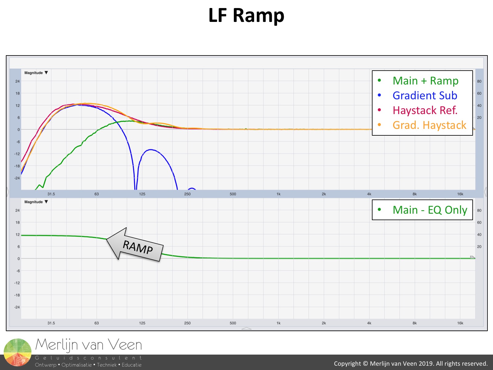 figure 7It’s now up to the mains to restore the missing content by “ramping” into the “haystacked” cardioid gradient array which can be achieved in several ways, e.g., by applying a low-shelf filter to the mains (figure 7).
Notice that the combined response, after applying the ramp, is in good agreement with the reference-haystack or target-curve. The remaining ripple is inevitable but by no means unacceptable.
As a bonus, you might actually like this aproach because the mains' direct radiators are typically less inert than those found in subwoofers.
That being said, over the years, I’ve become increasingly convinced that haystacking subwoofers whose bandwidth has been reduced by the gradient technique, is the predominant reason for the perceived lack of impact which brings us to next prejudice: time smearing.
Time Smearing
In the video below, I use tone bursts (gated sine waves) which are transient signals with a crest factor of 7,3 dB and a bandwidth of one-third octave, to demonstrate that time smearing is functionally inaudible, provided you limit yourself to the gradient array's usable frequency range (figure 2)!
The remaining spectrum is out-of-bounds where destructive interference will occur!
The tone bursts have been level-matched between the regular and gradient deployed arrays to eliminate any level-induced bias. Also notice that the average (RMS) difference with pink noise between both approaches is 1 dB at most.
Given the frequency range of interest, I encourage you to use headphones or a full-range loudspeaker system.