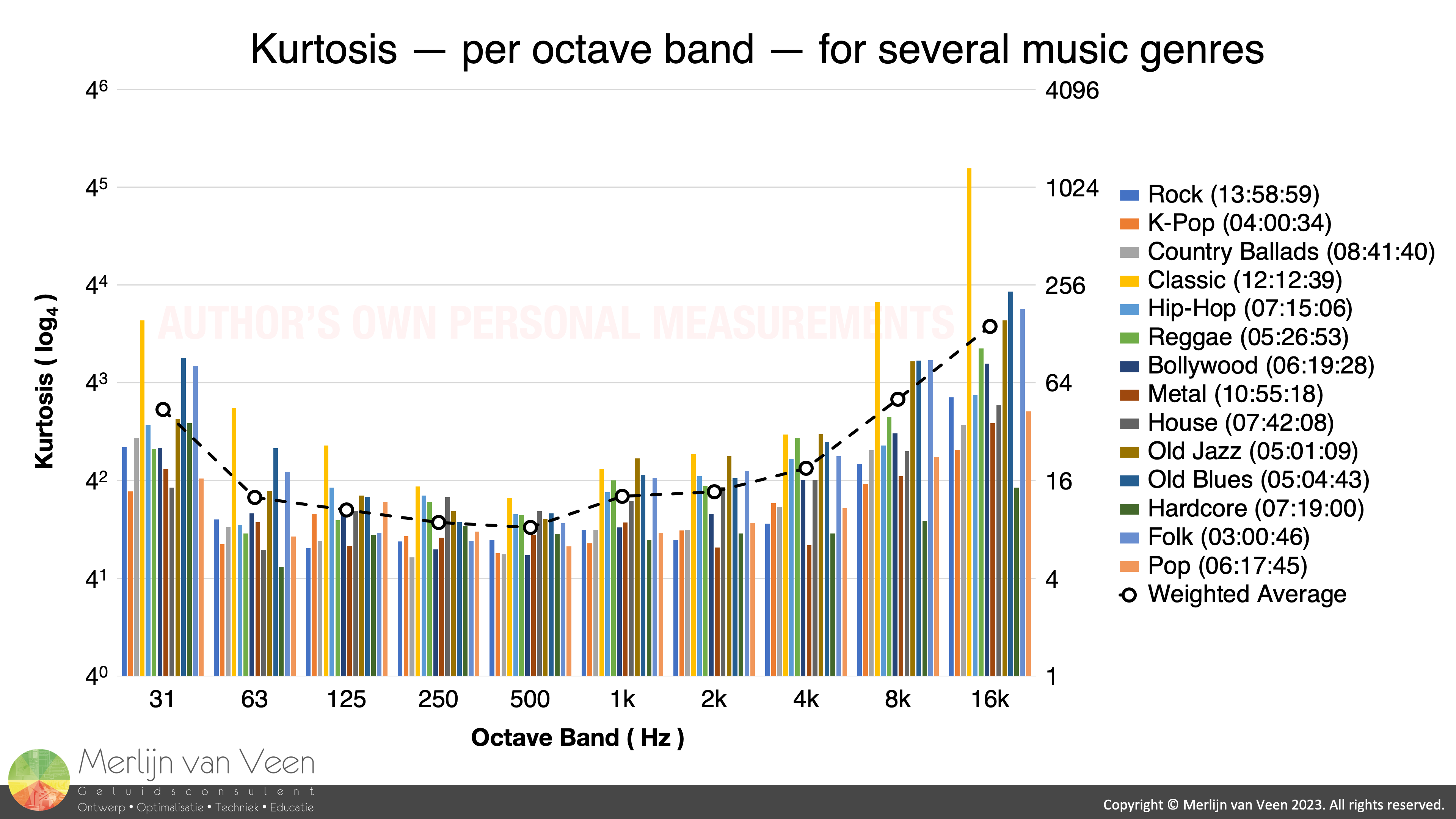
Figure 1Kurtosis and crest factor are closely related. But unlike crest factor, Kurtosis is not exclusively peak‑centric. Kurtosis indicates the presence of outliers in general as well as peaks. For music, kurtosis is a function of frequency (Figure 1).

Regrettably, in order to appreciate this, some math is inevitable.

"Which king loved fractions? Henry the ⅛."

The equation for kurtosis (\(\kappa\)) is:

\begin{equation}\kappa=\frac{1}{n}\sum_{i=1}^{n}\left ( \frac{\left [ x_i-\bar{x} \right ]}{s } \right )^4\end{equation}
Where \(x_i\) is the value of a single sample, \(\bar{x}\) is the samples' mean, \(s\) the samples' standard deviation, and \(n\) the number of samples.

The equation for standard deviation is:

\begin{equation}s=\sqrt{\frac{1}{n}\sum_{i=1}^{n}\left ( x_i-\bar{x}\right )^2}\end{equation}
No DC Offset

For audio — without a DC offset — the mean is zero. In which case Equation 2 simplifies to:

\begin{equation}s_{\,\bar{x}_{0}} =\sqrt{\frac{\left ( x_1^2+x_2^2+\cdots +x_n^2\right )}{n}}=RMS\end{equation}
Which is how we compute RMS levels for discrete signals (Part 1).

If we substitute Equation 3 into the denominator of Equation 1 with a mean of zero,
we get:

\begin{equation}\kappa_{\,\bar{x}_{0}}=\frac{1}{n}\sum_{i=1}^{n}\left ( \frac{x_i}{RMS} \right )^4\end{equation}
Expressed in words this means that, Kurtosis averages the ratio, of — each — sample's value with respect to the RMS level, raised to the fourth power.

Bearing in mind that, when the absolute value (sign insensitive) of a sample reaches a maximum, i.e., a peak, we can determine the crest factor (Part 1):

\begin{equation}Crest\,Factor=\frac{\left | x_{peak} \right |}{RMS}\end{equation}
Notice the similarity between just the fractions \(x_i\div RMS\) and \(x_{peak}\div RMS\) in Equations 4 and 5 respectively. Except that, Kurtosis considers — each — sample’s value. Whereas crest factor solely focuses on the loudest one. As such, it should not come as a surprise that Kurtosis and crest factor are closely related.

Quartic Growth

In Equation 4, raising the ratio \(x\div RMS\), of a sample's value (\(x_i\)) with respect to the RMS level, to the fourth power, has two vast implications:

• When a sample's value exceeds the RMS level, i.e., the ratio > 1.
  Raising the ratio to the fourth power, will make it grow dramatically.
  
  
• Whereas when the sample's value is less than the RMS level, i.e., the ratio < 1.
  Raising the ratio to the fourth power, will make it tend to zero.

Figure 2Figure 2 shows the massive impact of quartic growth (raising to the fourth power). Where both \(x\) and \(y\) axes are scaled logarithmically.

When a sample's value is four times the RMS level, as expected of peaks in, e.g, pink noise, it maps to a value of 256.

Whereas for sample values that are merely \(\sqrt{2}\) (≈1,41) times the RMS level, as expected of the "peaks" in a pure tone, they map to a value of merely four...

Samples whose value is less than the RMS level, effectively get zeroed out. And as such — contrary to the outliers and peaks — are of little consequence to the mean or average, i.e., kurtosis.

Examples

Figure 3Figure 3 shows the results for samples of a pure tone with crest factor \(\sqrt{2}\) (≈1,41) or 3 dB. Samples pulled from a uniform distribution with crest factor \(\sqrt{3}\) (≈1,73) or 4,8 dB. And samples pulled from a (bounded) normal distribution with crest factor 4 or 12 dB.

For each example, signal level has been normalized such that the RMS level has a value of one. Signal amplitude is shown on a linear scale. Whereas \((x_i\div RMS)^4\) — because of the quartic growth — is shown on a logarithmic scale (base 4).

Notice that as "outliers" rise in amplitude, Kurtosis — the mean of \((x_i\div RMS)^4\) — gains market share.

Mean or Median?

Raising \(x\div RMS\) to the fourth power can significantly skew the results' value‑distribution. So why then use an average for Kurtosis as opposed to the median?

For, e.g., income, it is well known to use the median — as measure for central tendency — rather than the mean. In such a scenario, using the mean would be ill‑advised. Because a single millionaire (rare outlier) could greatly bias the mean.

Whereas Kurtosis is deliberately all about — outliers — hence the mean as opposed to the median. And when data is — positively skewed — the mean will be larger than the median. To appreciate why, let us leverage "box‑and‑whisker" plots. Which offer a lot of insight, at a glance, especially for skewed data.

Figure 4Figure 4, shows "box‑and‑whisker" plots — albeit on a logarithmic scale — for a 1000‑sample‑long pure tone, a uniform‑distributed noise, and a normal‑distributed noise.

For the pure tone, there are no outliers. Whereas for the uniform‑distributed noise, roughly 6% of the samples are outliers. However, for the normal‑distributed noise, roughly 16% of the samples are outliers.

As the number of outliers ­and their amplitudes rise, the mean unambiguously starts to drift away from the median towards the outliers. And when kurtosis rises, whereby indicating more and taller outliers — including peaks — crest factor follows in lockstep.

When one passes music through a filter bank, consisting of ten 1‑octave‑wide band‑pass filters, and — for each octave — measures the kurtosis of the filtered signal. You get data like is shown in Figure 1. Subsequently, crest factor has to be a function of frequency as well.

Oftentimes, a rise in crest factor leads to the assumption that peaks got louder. While failing to realize that, if peak levels remain constant — while RMS levels drop — crest factor would rise as well!

AES75 Music‑Noise

Figure 5AES75 Music-Noise, a signal that simulates program content, (to the best of the author's knowledge) is the first test signal whose crest factor rises with increasing frequency. Like actual music.

Whereas other accepted simulated program content (IEC 60268‑1, ANSI/CTA 426‑B, or ANSI/CEA 2034‑A) are essentially spectrally‑shaped, i.e., equalized, pink noises. As such, like pink noise, their crest factor remains virtually constant with increasing frequency.

AES75 Music‑Noise is part of a recent standard for determining maximum linear sound levels of loudspeakers and loudspeaker systems (first published in 2022). In which case it is important that the simulated program content, i.e., test signal, simulates — both — the dynamic properties as well as spectrum expected of music.

For more information visit the AES75 website, or join the Official AES75 Facebook group.